Twenty robots move more than fifteen. That sounds self-evident enough that most planning documents never check it, and it holds only up to a point. Past it, every additional mobile robot contributes less, and eventually it lowers throughput outright. That point exists in every layout, though in many it sits beyond any fleet anyone would realistically buy. Where it sits depends on five properties of the layout, which is where every rule of thumb fails.
Why throughput does not scale with fleet size
An additional robot brings transport capacity and interactions at once. Capacity grows linearly: each robot adds its own transport performance. Interactions grow faster, because every new robot can conflict with every robot already there. It occupies edges, crosses the same intersections and queues at the same stations. What looks like a sum in a spreadsheet is a web of mutual obstruction in operation.
A mobile robot does not occupy a point, it occupies its own contour plus a margin. In our simulation that area is projected forward onto nodes and edges like an envelope, enlarged by overhanging loads. Ahead of it sits the protective field of the safety scanner, whose length follows the vehicle kinematics because it has to cover the stopping distance: faster driving means a longer field, and in a curve it shifts sideways. The space a robot claims therefore grows with its speed. The field stays a safety function on the vehicle; for throughput what counts is how far it reaches. The more robots move, the more often those areas overlap, and every overlap costs time.
The effect is documented, and it arrives earlier than most expect. In a simulation study of warehouse layouts with automated guided vehicles, throughput under a deadlock prevention strategy fell once the fleet passed roughly five to seven AGVs, because average waiting time per transport order rose faster than the capacity being added (Müller et al., Winter Simulation Conference 2020). So the rule set matters: a traffic rule that behaves unremarkably with a small fleet produces blocking once the fleet grows.
In short: The question is not how many robots fit into the building, it is at which robot the building starts getting slower.
The three ranges of the throughput curve
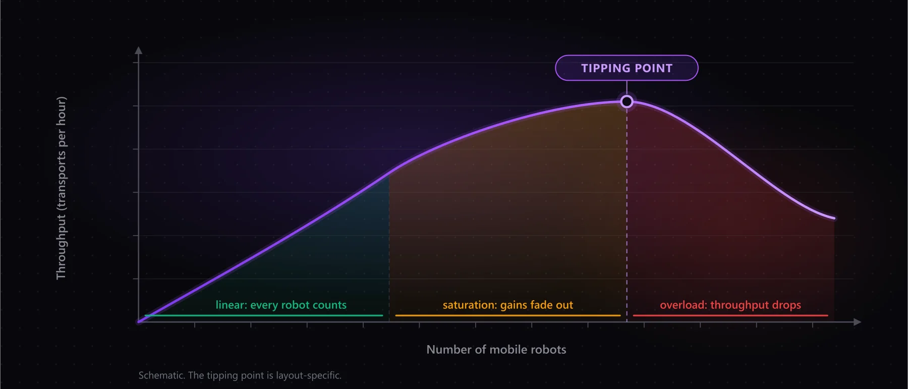
Plot transport performance against fleet size and three ranges appear. Which range a facility sits in decides whether another robot buys anything.
The linear range. Every additional robot raises throughput by almost its full contribution, because paths are clear enough that encounters stay rare. Even a back-of-the-envelope calculation holds here.
Saturation. The increment shrinks. An additional robot may deliver half or a third of its nominal contribution, the rest absorbed by waiting. Here it is decided whether one more robot still earns its cost.
Overload. Throughput falls. Additional robots block more than they contribute, while the fleet still looks busy: high utilisation, plenty of movement, declining performance at the stations.
The transition is rarely a sharp break and gets misread accordingly: more robots are ordered, and the result comes out worse than expected.
Five factors that move the tipping point
The tipping point is set by the path network the fleet drives through, not by the fleet itself.
- Narrow sections and one-way segments. A segment only one robot can use at a time acts like a valve. Two extra passing places can move the tipping point further than two extra robots.
- Intersections and right-of-way logic. The rule decides how long the waiting lasts. One favouring the main flow behaves differently under load than one resolving by arrival order.
- Stations and their queues. Sources and sinks have a finite processing time. A queue in front of one grows into an aisle and blocks traffic unrelated to it.
- Contours, protective fields and overhanging loads. Large load carriers enlarge the envelope and the space each robot needs, with the speed-dependent protective field in front of that. The same hall carries a bigger fleet with small, slow robots than with fast ones and overhanging pallets.
- Charging and availability. Charging robots are part of the traffic. They drive to the charging point, may queue there and occupy corridors, so the charging concept moves the tipping point too.
These five appear on no data sheet, yet belong in any model a fleet size comes out of.
Why no rule of thumb hits the point
Rules like “so many robots per thousand square metres” or “so many transports per robot and hour” fail reliably: they describe the fleet, while the path network sets the tipping point. Two halls of identical area and volume can differ widely, because one has two loops and the other a dead end.
A second difficulty: fleet size is often supplied by the vehicle vendor, the party that earns on selling more robots. You will rarely hear “beyond this point another robot adds nothing” from that direction. Why static calculations hit their limits with mobile robots, we covered in Simulate before you invest.
How to find the tipping point before you buy
Test fleet size as a series, not a single value. In simulation that looks like this:
- Import the layout and build the path network. The hall plan usually exists as a DXF. Nodes, edges, corridors, stations and the traffic rules are built on top of it.
- Run fleet size as a series. Not one run at the planned number, but a sequence with rising fleet size. The result is a curve.
- Test at peak load and across several days. Typical studies run several days up to a full week continuously, usually at 110 to 120 percent of planned load. The range just before the tipping point is sensitive, and a sample day will not show it.
- Read the shape of the curve. What matters beyond the tipping point is how flat the curve runs before it. A very flat saturation means the last two robots barely contribute, which is a procurement decision.
- Move the point. Pause the run, add a passing place, change a right-of-way rule, relocate a station, start again. The run is discrete and repeatable, so every change is measured against the same starting state: build, evaluate, rebuild, evaluate, much like in a game engine. The layout improves step by step instead of in one big throw.
The simulation is graph-based, working with nodes, edges and corridors as described by LIF and VDA 5050. That matches our own projects: in structured intralogistics even autonomous mobile robots usually travel on virtual path networks, because free navigation makes throughput hard to predict. Free-roaming SLAM systems without a defined path network are out of scope.
Conclusion
- Throughput does not scale linearly with fleet size: capacity grows linearly, interactions grow faster.
- Every facility has a tipping point beyond which extra robots reduce transport performance. Whether it sits within reach is decided by the layout.
- The point belongs to the path network. Narrow sections, intersections, stations, contours with their protective fields and the charging concept all move it.
- If the throughput target sits beyond it, the answer is a layout change, not a larger order.
- None of this shows up unless fleet size is studied as a curve, at peak load, across several days.
Planning a fleet and wondering at which robot your layout starts getting slower? In a free initial call we work out that curve for your facility, get in touch. Our planning page shows how such a study runs.

About the author
Tim Nowak
Tim Nowak is co-founder and Managing Director of ScaliRo GmbH. He supports operators, manufacturers and integrators with vendor-independent planning and simulation of mobile robot fleets.
LinkedIn